Next: 7 Conventions Up: dev_guide Previous: 5 Apps Contents
The Test Harness is a flexible test control system intended to provide a thorough parameter space exploration of remapping and redistribution of distributed arrays and fields. The parameter space is defined through configuration files which are interpreted at run time to perform the desired tests.
The Test Harness is integrated into the Unit test framework, enabling the Test Harness to be built and run as part of the Unit tests. The test results are reported to a single standard-out file which is located with the unit test results.
The motivation for employing such a hierarchy configuration files is to allow a high degree of customization of the test configurations by combining individual specification files. Complex combinations of test cases are easily specified in high level terms. Each class will have its own collection of specification files tailored to the needs of that class.
There are three ways to invoke the test harness, as an integral part of running unit tests; as a stand-alone test invoked through gmake; and as a standalone test invoked through the command line.
Running the harness along with the unit tests provides frequent regression testing of the redistribution and regridding features.
Running the test harness in stand alone mode using gmake is useful for isolating faults in failed test cases.
Running the test harness from the command line provides the most control over Test Harness execution. Understanding the underlying program allows the developer full access to test harness features. This is useful in developing makefiles, scripts, and configuration files.
The environment variables currently defined are:
The targets currently supported for the ESMF_TESTHARNESS_ARRAY variable are:
The targets currently supported for the ESMF_TESTHARNESS_FIELD variable are:
Each target selects the desired sequence of test cases for that target. For example, a series of test cases could be developed to run on different days providing partial test coverage on a particular day, but complete coverage over a week. In this case, each day would have a separate target and the environment variable would be set for that day's test case.
An example of a test harness appears below.
RUN_ESMF_TestHarnessField_1:
	\$(MAKE) TESTHARNESSCASE=field_1 NP=4 run_test_harness
In this example, the test harness target is RUN_ESMF_TestHarnessField_1. This target will execute a single test harness test case. Additional lines can be added if additional steps are desired. The next section will describe the details of invoking a test case.
For example,
gmake TESTHARNESSCASE=field_1 NP=4 run_test_harnesswill run the test harness test case, field_1 on 4 processors.
Each test case is defeined by a series of configuration files in the <classdir>/tests/harness_config directory. All of the configuration files for a particular test case will be prefixed with <casename>_ where <classname> is a unique name for the test. The top level configuration file will have a suffix of _test.rc. Thus, the top level configuration file for the field_1 test case will be field_1_test.rc.
The next section describes invoking the Test Harness from the Command Line.
To run the executable, enter:
\<run path\>ESMF\_TestHarnessUTest \<cmd args\>
where,
\<run path\> is the path to the executable,
and \<cmd args\> are the optional command arguments

The cmd args are as follows:
-path \<config path\>
-case \<case filename\>
-xml \<xml filename\>
-norun
The path argument sets the path to the configuration files. All of the configuration files for a testcase must reside in the same directory. If this argument is not present, the current working directory will be used as the path.
The case argument is the name of the top level configuration file. This is described in a later section of this document. If this argument is not present, test_harness.rc will be used.
The xml argument instructs the test harness to generate an XML test case summary file in the current working directory.
The norun argument instructs the test harness not to run the test cases. The configuration files will be parsed and if selected, an XML file will be generated. The XML file can be post-processed to generate human readable test configuration summary reports.
If running under mpi, you would need to prefix this command with the proper mpirun command.
The next section describes the format of the top level resource file.
The top level configuration file specifies the test class, the format for reporting the test results, and the location and file names containing the problem descriptor files.
Originally, the test harness had a single configuration file for each class and supported only two test cases, a non-exhaustive case and an exhaustive case. This turned out to be too restrictive and test cases are now selected through environment variables. Unfortunately, some of the old constructs remain until the obsolete feature is removed.
Currently, the test harness only uses the non-exhaustive test case for each configuration file. So, referencing the example below, only the nonexhaustive tag is actually used by the test harness.
Also note, that comments are preceded by the # sign, that single parameter values follow a single colon : punctuation mark, while tables of multiple parameter values follow, and are terminated by, a double set of colon :: punctuation marks. This file is read by the ESMF_Config class methods, therefore must adhere to their specific syntax requirements. The entries can be in any order, but the name tags must be exact - including CAPITALIZATION. While it is not strictly necessary, the file names are enclosed in quotation marks, either single or double, to guarantee they are read correctly.
# Field test Harness Config file

# test class
test_class: FIELD

# report a summary of the test configurations before actually conducting tests
setup_report: TRUE

# test result report - options are:
# test_report: FULL  - full report presenting both success and failure configs
# test_report: FAILURE - report only failure configurations
# test_report: SUCCESS - report only successful configurations
# test_report: NONE - no report
test_report: FAILURE

# descriptor file for the nonexhaustive case
nonexhaustive::
   'nonexhaustive_descriptor.rc'
::   # end of list

# descriptor files for the exhaustive case (obsolete, but keep in for awhile)
exhaustive::
   'exhaustive_descriptor.rc'
:: # end of list
The argument for the tag test_class: specifies the ESMF class to be tested. Here it is Field.The tag setup_report: specifies if a setup report is sent to the test report. The tag test_report: specifies the style of report to be constructed. This report is appended to the standard-out file which is located with the Unit test results. The tag nonexhaustive:: delimits a table which contains the file names of problem descriptor files pertaining to the current test configuration.
The tag exhaustive is obsolete and will be removed when time permits. It has been replaced with the Test Harness environment variables which can select the desired test case from the available portfolio.
The problem descriptor files contain descriptor strings that describe the family of problems with the same memory topology, distribution, and grid association. The files also contain the names of specifier files which complete the descriptions contained within the descriptor strings. This structure allows a high level of customization of the test suite.
The problem descriptor file contains only one table, again conforming to the ESMF_Config class standard. The contents of the table must be delimited by the tag problem_descriptor_string::. The first element on the line, enclosed by quotes, is the problem descriptor string itself. Since the descriptor strings contain gaps and special characters, it is necessary to enclose the strings in quotation marks to guarantee proper parsing. The problem descriptor table may contain any number of descriptor strings, up to the limit imposed by the ESMF_Config class, each on a new line. Lines can be continued by use of an ampersand & as a continuation symbol at the beginning of any continued line. The syntax of the problem descriptor string follows the field taxonomy syntax. The following is a basic redistribution example.
# Basic redistribution example
#####################################
problem_descriptor_string::
'[B1G1;B2G2] --> [B1G1;B2G2]'  -d Dist.rc -g Grid.rc
'[B1G1;B2G2] --> [B1G2;B2G1]'  -d DistGrid.rc
 & otherDistGrid.rc yetanotherDistGrid.rc
 &  -g Grid.rc anotherGrid.rc
::   # end of list
In the above example, the two problem descriptor strings specify that a redistribution test is to be conducted, indicated by the syntax ->, between a pair of rank two blocks of memory. Following the problem descriptor string, are multiple flags and the names of specifier files. Each flag indicates a portion of the configuration space which is defined by the contents of the indicated specifier files.
| argument | definition |
| -d | DELayout/DistGrid specification |
| -g | Grid specification |
For example
![]() indicates that a 2D logically rectangular block of memory
is associated with a 2D grid in its natural order.
The signifier
indicates that a 2D logically rectangular block of memory
is associated with a 2D grid in its natural order.
The signifier ![]() represents an undistributed tensor grid.
Reversing the grid signifiers
represents an undistributed tensor grid.
Reversing the grid signifiers ![]() indicates that the fastest varying dimension
is instead associated with the second grid dimension.
Specific information about the grid, such as its size, type, topology are left to be defined
by the specifier files. It is the associations between memory and the grid that are stressed with this syntax.
indicates that the fastest varying dimension
is instead associated with the second grid dimension.
Specific information about the grid, such as its size, type, topology are left to be defined
by the specifier files. It is the associations between memory and the grid that are stressed with this syntax.
To distribute the grid, a distribution signifier is needed.
The block distribution of each memory dimension is indicated by the signifier ![]() .
Therefore
.
Therefore
![]() signifies that a 3D logically rectangular block of memory,
which has a 3D associated grid, is distributed in its first two dimensions, and not its third.
signifies that a 3D logically rectangular block of memory,
which has a 3D associated grid, is distributed in its first two dimensions, and not its third.
As an example, consider a block of memory. To associate a tensor grid with specific dimensions of that block,
the symbol ![]() is used with a numerical suffix to indicate a specific dimension of the grid.
The specific aspects of this grid are left undefined at this point, only the fact
that a particular dimension of a grid is associated with a particular dimension
of the memory block is implied by the grid syntax.
is used with a numerical suffix to indicate a specific dimension of the grid.
The specific aspects of this grid are left undefined at this point, only the fact
that a particular dimension of a grid is associated with a particular dimension
of the memory block is implied by the grid syntax.
The complete syntax for a tensor grid specification is
![]() where
where
To illustrate the use of this syntax consider the following example.
[ G1 ; G2 + H{1:1} ]
At times a memory location might have no grid association.
The symbol ![]() is used in this case as a place holder. For example,
is used in this case as a place holder. For example,
[ G2 ; G1 ; * ]
In this example, the grid association has been reversed from from its natural order. The first memory location is associated with the second grid dimension, and the second memory location with the first grid dimension.
As was mentioned before, the symbol ![]() is used as a place holder to indicate a lack of association.
If the third memory location of an undistributed block of memory has no grid association, it would look like this;
is used as a place holder to indicate a lack of association.
If the third memory location of an undistributed block of memory has no grid association, it would look like this;
[ G1; G2; * ]
[ B1 G1; B2 G2; * G3 ]
Lastly, if the last memory location has no associations, it would look like;
[ B1 G1; B2 G2; * * ]
| Action | |
| B | first order bilinear interpolation |
| P | patch recovery interpolation |
| C | first order conservative interpolation |
| S | second order conservative interpolation |
| N | nearest neighbor distance weighted average interpolation |
| X | unknown or user provided interpolation |
The problem descriptor string
[B1 G1; B2 G2 ] --> [B1 G1; B2 G2 ]
Alternatively the example
[ B1 G1; B2 G2 ] =C=> [ B1 G1; B2 G2 ]
[ B1 G1; B2 G2 ] @{#,#}
The stagger location key represents the location of a field with respect to the cell center location. It is indicated by relative cartesian coordinates of a unit square, cube etc. To illustrate this further, consider the example of a 2D grid. The cell is represented by a unit square with the xy axis placed at its center, with the positive x-axis oriented East and the positive y-axis oriented North. The actual values are suppressed, only the directions ![]() , and
, and ![]() are used. This geometry is for reference purposes only, and does not literally represent the shape of an actual cell.
are used. This geometry is for reference purposes only, and does not literally represent the shape of an actual cell.
The cell center, located at the origin of the cell, is indicated by ![]() . The corner of the cell is indicated by
. The corner of the cell is indicated by ![]() , where the ones have been dropped to just leave the plus signs. The cell face normal to the X axis (right wall) is indicated by
, where the ones have been dropped to just leave the plus signs. The cell face normal to the X axis (right wall) is indicated by ![]() , while the face normal to the Y axis ( top wall) is indicated by
, while the face normal to the Y axis ( top wall) is indicated by ![]() . This approach generalizes well to higher dimensions.
. This approach generalizes well to higher dimensions.
| argument | definition |
| Center | { 0,0 } |
| Corner | { +,+ } |
| Face normal to X axis | {+,0 } |
| Face normal to Y axis | {0,+ } |
With these four locations, it is possible to indicate the standard Arakawa grid staggerings. A key of ![]() would be equivalent to an Arakawa A-grid, while a key of
would be equivalent to an Arakawa A-grid, while a key of ![]() would represent an Arakawa B-grid. Components of the C and D grids would be indicated by wall positions
would represent an Arakawa B-grid. Components of the C and D grids would be indicated by wall positions ![]() and
and ![]() .
.
| Grid Stagger | coordinates |
| A-grid | { 0,0 } |
| B-grid | { 1,1 } |
| C-grid & D-grid | { 0,1 } and { 1,0} |
For example, the string
[B1 G1; B2 G2 ] =C=> [B1 G1; B2 G2 ] @(+,+)indicates that a collection of regridding tests are to be run where a block distributed two dimensional field, is interpolated from one two dimensional grid onto a second two dimensional grid, using a first order conservative method. The source field data is located at the cell centers (an A-grid stagger location) and the destination field is to be located at north east corner (a B-grid stagger location). Additional information about the pair of grids and their distributions must be specified to run an actual test.
This process generalizes to higher dimensions. Consider
[B1 G1; B2 G2 ; G3 ] =C=> [B1 G1; B2 G2 ; G3 ] @(+,+,+)indicates that a collection of regridding tests are to be run between a 3D source grid (cell centered) and a 3D destination grid where the field stagger location is the upper corner of the 3D cell (B-grid horizontally and top of the cell vertically).
A further discussion on grid staggers can be found in section on the ESMF Grid class in the Reference manual.
For example, in models with nested grids or which employ multi-grid methods, it is useful to have an indexed structure of logically rectangular blocks of memory, where each block is generally a different shape and size. Such a structure can be represented with parentheses as delimiters, such as
( tile , [ B1 G1; B2 G2 ] )
The nature of the grid specifier file varies depending on whether the test is a redistribution or a regridding. A redistribution test takes a field associated with a grid and rearranges it in processor space. So while a source and destination distribution are needed, only a single grid is necessary to conduct the test. A regridding test, on the other hand, takes a field associated with a source grid and interpolates it to a destination grid thaty is also part of a field. In this case both source and destination grids are needed. It is also assumed that a source and destination distribution is specified.
| Redistribution | source grid |
| source & destination distribution | |
| Regridding | source & destination grids |
| source & destination distribution |
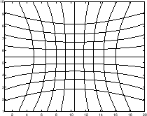
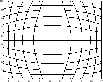
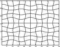
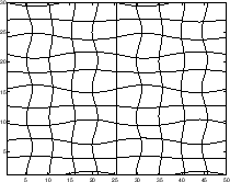
The first step of the grid generation is to generate a rectilinear grid of specified size, range of coordinates, and either uniform or gaussian spacing between the coordinates. If only a rectilinear grid needed, the grid generation is finished. If a curvilinear grid is desired, the rectilinear grid is taken as a base grid and its coordinates are smoothly stretched and/or shrunk according to an analytical function, to produce a curvilinear mesh according.
| key word | formula
|
| contracting |
|
|
|
|
| expanding |
|
|
|
|
| symmetric_sin |
|
|
|
|
| asymmetric_sin |
|
|
|
These four choices for ![]() equate into four options for analytically generated curvilinear grids.
equate into four options for analytically generated curvilinear grids.
Examples of these four curvilinear grid options are plotted in figure ![[*]](crossref.png) .
.
|
This adds up to a total of 2 types of rectilinear grids (uniform and gaussian), each with three options (no connection, spherical pole connection, and a periodic option). A large variety of grids can be formed by mixing and matching the grid types and options. For example a standard latitude-longitude grid on a sphere is formed by using the pair of grid types uniform_periodic and uniform_pole. A gaussian grid is formed with uniform_periodic and gaussian_pole. And a regional grid on a sphere, without periodicity, with uniform and uniform. A summary of the rectilinear grid types is given below.
| Rectilinear grid options | |
| grid type | modifier |
| UNIFORM | none |
| _POLE | |
| _PERIODIC | |
| GAUSSIAN | none |
| _POLE | |
| _PERIODIC | |
The various curvilinear grid types are created in the same way of mixing and matching grid type options. A regional expanding grid is formed using the grid types expanding and expanding. Likewise a rotated regional grid is created by using the grid types rotation_15degrees and rotation_15degrees to indicate the grid type. A summary of the curvilinear grid types is given below.
| Curvilinear grid options | |
| grid type | modifier |
| CONTRACTING | none |
| _POLE | |
| _PERIODIC | |
| EXPANDING | none |
| _POLE | |
| _PERIODIC | |
| SYMMETRIC_SIN | none |
| _POLE | |
| _PERIODIC | |
| ASYMMETRIC_SIN | none |
| _POLE | |
| _PERIODIC | |
| rotation_15degrees | none |
| rotation_30degrees | none |
| rotation_30degrees | none |
| parameters to define a grid for redistribution |
| Grid rank |
| Grid dimensions |
| Range of the coordinate axis |
| Coordinate units |
This is the information is provided by the redistribution grid specifier file. An example of a redistribution grid specifier file is provided below.
# grid.rc
########################################
map_type: REDISTRIBUTION

# regular rectilinear Grid specification
map_redist::
#rank spacing  size  range (min/max)  units
#
2  'UNIFORM'  120  -3.14159  3.14159  'RAD'   'UNIFORM'  90  -1.57  1.57  'RAD'
#
2  'UNIFORM'  400  -180   180  'DEG_E'  'GAUSSIAN'  200 -88   88   'DEG_N'
::
The first piece of information required for the file is the map_type key. It should be set to REDISTRIBUTION to indicate that it is intended to define grids for a redistribution test. Next is a configuration table which specifies multiple grids. The specification can be stretched over multiple table lines by use of the continuation symbol ![]() . The order of information is as follows:
. The order of information is as follows:
| parameters to define a grid for redistribution |
| Grid rank |
| Grid axis type |
| Grid size |
| Range of the coordinate axis |
| Coordinate units |
There are two 2D grids specified in the file. The first is a standard uniformly spaced latitude-longitude grid, where none of the grid coordinates has any topological connections. The horizontal coordinates are in radians. The second 2D grid is a gaussian spherical grid. The gaussian grid has a spherical topology and is in degrees.
Four types of coordinate units are supported; degrees, radians, meters and kilometers. Each has multiple equivalent key words.
| Supported units | |
| name | key word |
| Degrees | DEGREES |
| DEG | |
| DEG_E | |
| DEG_N | |
| Radians | RADIANS |
| RAD | |
| Meters | METERS |
| M | |
| Kilometers | KILOMETERS |
| KM | |
| parameters to define a grid for remapping |
| source and destination grid rank |
| source and destination grid axis type |
| source and destination grid dimensions |
| source and destination range of coordinate axis |
| source and destination coordinate units |
| test function with parameters to interpolate |
This information is provided by the regridding grid specifier file. An example of a regridding grid specifier file is provided below.
# grid.rc
########################################
map_type: REGRID

################################################################################
# grid | source | grid    |    grid   | grid  | units | destination |
# rank |  tag   | spacing | dimension | range |       |    tag      |
################################################################################
# Grid specification for regridding

#rank spacing  size  range (min/max)  units
map_regrid::
# example of a pair of 2D periodic grids
2   SRC    UNIFORM_PERIODIC   120   -3.14159  3.14159  RADIANS
&              UNIFORM_POLE             90    -1.57        1.57        RADIANS
&   DST    UNIFORM_PERIODIC   120  -180      180             DEG_E
&              GAUSSIAN_POLE           88    -88        88             DEG_N
&   FUNCTION    CONSTANT   2.1 0.1  END
::
The first piece of information required for the file is the map_type key. It should be set to REGRID to indicate that it is intended to define grids for a regridding test. Next is a configuration table which specifies multiple pairs of grids. The specification can be stretched over multiple table lines by use of the continuation symbol ![]() . The order of information is as follows:
. The order of information is as follows:
| parameters to define a grid for reremapping |
| Grid rank |
| Source grid axis type |
| Source grid size |
| Source range of the coordinate axis |
| Source coordinate units |
| Destination grid axis type |
| Destination grid size |
| Destination range of the coordinate axis |
| Destination coordinate units |
| Test function and parameters |
The regridding grid specifier file contains a pair of 2D grids. The source grid is a standard latitude-longitude grid on a spherical topology. The destination grid is a spherical gaussian grid also on a spherical topology. The source grid is in radians, while the destination grid is in degrees. The test function is a periodic function of the grid coordinates.
The one new piece of information for the regridding specifier files are the predefined test functions. The test functions provide a physical field to be interpolated and are generated as an analytical function of the grid coordinates. Supported options include:
| Test functions | ||
| name | function | parameters |
| constant | set value at all locations | value, relative error |
| coordinate | set to a multiple of the coordinate values | scale, relative error |
| spherical harmonic | periodic function of the grid coordinates | amplitudes and phases, relative error |
The CONSTANT value test function sets the field to the value of the first parameter following the name. The second value is the relative error threshold. For example, the test function specification:
& FUNCTION CONSTANT 2.1 0.1 END
indicates that the field is set to the constant value of ![]() , with a relative error threshold
of
, with a relative error threshold
of ![]() . This test function specification holds for grids of any rank.
. This test function specification holds for grids of any rank.
The COORDINATE test function sets the field to the value of the one of the grid coordinates multiplied by the value of the first parameter following the name. The second value is the relative error threshold. For example, the test function specification:
& FUNCTION COORDINATEX 0.5 0.1 END
indicates that the field is set to one half of the X coordinate values. For a 2D grid the coordinate options include COORDINATEX and COORDINATEY. For a 3D grid there is the additional option of COORDINATEZ. Again, the relative error threshold is ![]() .
This test function specification holds for grids of any rank.
.
This test function specification holds for grids of any rank.
The SPHERICAL_HARMONIC test function sets the field to the periodic harmonic function
![]() .
The parameters follow the order
.
The parameters follow the order
& FUNCTION SPHERICAL_HARMONIC a kx b ly rel_error END
This test function specification is only valid for 2D grids.
Here is an example of a distribution specification file for block and block cyclic distributions.
##################################################
# descriptive | source | source | operator | destination | dest | operator | end
# string      |  tag   |  rank  |  & value |     tag     | rank | & value  | tag
##################################################

# table specifing 2D to 2D distributions
distgrid_block_2d2d::

# example with two fixed distribution sizes
 '(1,2)-->(2,1)'  'SRC' 2  'D1==' 1  'D2==' 2  'DST' 2  'D1==' 2  'D2==' 1  'END'

# example with one fixed and one variable distribution size
 '(1,n)-->(n,1)'  'SRC' 2  'D1==' 1  'D2=*' 1  'DST' 2  'D1=*' 1  'D2==' 1  'END'

# example with variable distribution sizes
 '(2n,n/2)-->(n/2,2n)'  'SRC'  2  'D1=*'  2    'D2=*'  0.5
 &                      'DST'  2  'D1=*'  0.5  'D2=*'  2     'END'

# another example with variable distribution sizes
 '(2n,n/2)-->(2n,(n/2)-1)'  'SRC' 2  'D1=*' 2  'D2=*'  0.5
 &                          'DST' 2  'D1=*' 2  'D2=*'  0.5  'D2=+' 1   'END'
::

# table specifing 3D to 3D distributions
distgrid_block_3d3d::

# example with two fixed distribution sizes
 '(1,2,1)-->(2,1,1)'  'SRC' 3  'D1==' 1  'D2==' 2  'D3==' 1
 &                    'DST' 3  'D1==' 2  'D2==' 1  'D3==' 1  'END'
::
| parameters to define a grid distribution |
| Descriptive string |
| Source key |
| Source distribution rank |
| Source distribution axis and size for each dimension of the distribution |
| Destination key |
| Destination distribution rank |
| Destination grid size |
| Destination distribution axis and size for each dimension of the distribution |
| Termination key |
The second example, illustrates how to indicate a scalable distribution. Again the entry ![]() indicates that the first dimension of the distribution is set to one, but the entry
indicates that the first dimension of the distribution is set to one, but the entry ![]() has a different meaning. It takes the total number of PETs NPETS and scales it by one. Therefore the source distribution becomes
has a different meaning. It takes the total number of PETs NPETS and scales it by one. Therefore the source distribution becomes
![]() . It automatically scales with the number of PETs. Likewise, the destination distribution is set to
. It automatically scales with the number of PETs. Likewise, the destination distribution is set to
![]() .
.
The third example is completely dynamic. Since both ![]() and
and ![]() are scalable, each dimension starts with
are scalable, each dimension starts with ![]() PETs, where
PETs, where ![]() is the square root of
is the square root of ![]() rounded down to the nearest integer. Therefore
rounded down to the nearest integer. Therefore
![]() . So if
. So if ![]() , Then
, Then ![]() . If
. If ![]() then
then ![]() still equals
still equals ![]() . This base value is then modified by the indicated entries. In this case the source distribution is
. This base value is then modified by the indicated entries. In this case the source distribution is
![]() , since the tag
, since the tag ![]() indicates that first dimension is the result of the base value being multiplied by two, and the second dimension is the result of the base value being multiplied by one half. Likewise, the destination distribution is set to
indicates that first dimension is the result of the base value being multiplied by two, and the second dimension is the result of the base value being multiplied by one half. Likewise, the destination distribution is set to
![]() , no matter the number of
, no matter the number of ![]() .
.
For a rank three scalable distribution, ![]() is the cube root of NPETS rounded down to the next integer. And so on for higher rank distributions.
is the cube root of NPETS rounded down to the next integer. And so on for higher rank distributions.
The fourth example illustrates the last option in the syntax. Again, since the distribution specifies two scalable distributions, ![]() is the square root of
is the square root of ![]() rounded down to the nearest integer. The source distribution is exactly the same as in the third example, but destination distribution has a new entry
rounded down to the nearest integer. The source distribution is exactly the same as in the third example, but destination distribution has a new entry ![]() . The first dimension of the destination distribution is set to
. The first dimension of the destination distribution is set to ![]() by the entry
by the entry ![]() . the second dimension is first set to
. the second dimension is first set to ![]() by the entry
by the entry ![]() , but then modified further to
, but then modified further to ![]() by the entry
by the entry ![]() . The resulting destination distribution is
. The resulting destination distribution is
![]() .
.
The syntax for modifying the size of the distribution space combines according to the order of the operations. The entries ![]() and
and ![]() , are not identical to
, are not identical to ![]() and
and ![]() , which would result in a dimension of size
, which would result in a dimension of size ![]() .
.
Three operations are supported:
| Distribution specification operations | |
| D# == | specify a fixed value |
| D# =* | multiply a base value by a constant |
| D# =+ | add a constant to the base value |
Consider a problem descriptor string consisting of two descriptor strings describing an ensemble of remapping tests.
[ B1 G1; B2 G2 ] =C=> [ B1 G1; B2 G2 ] @{+,+}
[ B1 G1; B2 G2 ] =B=> [ B1 G1; B2 G2 ] @{+,+}
Suppose the associated specifier files indicate that the source grid is rectilinear and is 100 X 50 in size. The destination grid is also rectilinear and is 80 X 20 in size. The remapping is conducted from the A-grid position of the source grid to the B-grid stagger of the destination grid. Both grids are block distributed in two ways, 1 X NPETS and NPETS X 1. And suppose that the first dimension of both the source and destination grids are periodic. If the test succeeds for the conservative remapping, but fails for one of the first order bilinear remapping configurations, the reported results could look something like
SUCCESS: [B1 G1; B2 G2 ] =C=> [B1 G1; B2 G2 ] @{+,+}
FAILURE: [B1{1} G1{100}+P; B2{npets} G2{50} ] =B=>
                         [B1{1} G1{80}+P; B2{npets} G2{20} ] @{+,+}
     failure at line 101 of test.F90
SUCCESS: [ B1{npets} G1{100} +P; B2{1} G2{50} ] =B=>
                         [ B1{npets} G1{80}+P; B2{1} G2{20} ] @{+,+}
[ B1{npets} G1{80}+P; B2{1} G2{20} ] @{+,+}
The report indicates that all the test configurations for the conservative remapping are successful. This is indicated by the key word SUCCESS which is followed by the successful problem descriptor string. Since all of the tests in the first case pass,there is no need to include any of the specifier information. For the second ensemble of tests, one configuration passed, while the other failed. In this case, since there is a mixture of successes and failures, the report includes specifier information for all the configurations to help indicate the source of the test failure.
The supplemental information, while not a complete problem description, since it lacks items such as the physical coordinates of the grid and the nature of the test field, includes information crucial to isolating the failed test.
esmf_support@ucar.edu