Regridding
Overview
Regridding, also called remapping or interpolation, is the process of changing the grid that underlies data values while preserving qualities of the original data. Different kinds of transformations are appropriate for different problems. Regridding may be needed when communicating data between Earth system model components such as land and atmosphere, or between different data sets to support operations such as visualization.
Regridding can be broken into two stages. The first stage is generation of an interpolation weight matrix that describes how points in the source grid contribute to points in the destination grid. The second stage is the multiplication of values on the source grid by the interpolation weight matrix to produce values on the destination grid. This occurs through a parallel sparse matrix multiply. ESMF can be run so that only interpolation weights are generated, or so that weights are both generated and applied, or so that weights that come from some external source can be read in and applied.
Ways to use ESMF Regridding
There are several ways to use ESMF regridding.
-
Fortran: Within Fortran code, such as in a coupled numerical model, ESMF regridding can be called to generate and apply interpolation weights. This is sometimes called “online” or “integrated” regridding. See the Field regridding section of the ESMF Reference Manual for more information on this option. The NUOPC Layer provides automatic regridding between components using Connector components.
-
Command line: Two command line appliations are installed with ESMF to generate and optionally apply interpolation weights from the command line using NetCDF files. These applications are ESMF_RegridWeightGen, which generates interpolation weights and ESMF_Regrid, which generates and applies interpolation weights.
-
Python: In Python scripts, the access to ESMF regridding capabilities is provided through ESMPy.
Regridding Options
Coordinate Systems
- Cartesian: Sometimes used for small regional grids. Coordinates expressed in terms of distance (e.g. x,y)
- Spherical: The standard spherical Earth representation. Coordinates expressed in angles. (e.g. longitude, latitude)
Grid Types
-
Grid/logically rectangular: A grid whose points could be stored in a rectangular index space, or a set of rectangular index spaces. Also sometimes called a structured grid. Examples of this type of grid include a regular latitude-longitude grid, and a cubed sphere grid. ESMF currently supports 2D or 3D logically rectangular grids:
- 2D: These grids consist entirely of quadrilaterals.
- 3D: These grids consist entirely of hexahedrons.
-
Mesh/unstructured: A superset of logically rectangular grids consisting of cells with possibly different numbers of sides connected together. An example of this is a grid with triangular cells. ESMF currently supports 2D or 3D meshes:
- 2D: ESMF supports meshes containing polygons with any number of sides (e.g. triangles, quadrilaterals, pentagons,…). Polygons with more than four sides are represented internally as a set of triangles, but to the user should behave as if they are a single polygon.
- 3D: ESMF supports meshes containing hexahedrons and tetrahedrons.
-
LocStream/location stream: A set of disconnected points. This option is useful for representing the locations of data where there is no inherent structure connecting the points into cells (e.g. a set of scattered observations). Because of the lack of cell structure, location streams are not appropriate as the source and destination for every regrid method.
Regridding methods
-
Bilinear: Linear interpolation in 2 or 3 dimensions.
-
Higher-order patch recovery (Patch): Patch rendezvous method of taking the least squares fit of the surrounding surface patches. This is a higher order method that may produce interpolation weights that may be slightly less than 0 or slightly greater than 1.
-
Nearest source to destination: Each destination point is mapped to the closest source point. A source point can be mapped to multiple destination points. Some source points may not be mapped.
-
Nearest destination to source: Each source point is mapped to the closest destination point. A destination point can be mapped to multiple source points, in which case the destination is the sum of the source values. Some destination points may not be mapped.
-
First-order conservative: Preserves the integral of the source field across the regridding. For this method, weight calculation is based on the ratio of source cell area overlapped with the corresponding destination cell area. If the user areas option (see below) is not used, then the areas used in this calculation are those calculated by ESMF and thus the ones for which the conservation holds. The user areas option allows the user to adjust the interpolation weights so that conservation is based on user-supplied areas.
-
Second-order conservative: Like first-order conservative, this method preserves the integral of the source field across the regridding. Also like the first-order, weight calculation is based on the ratio of source cell area overlapped with the corresponding destination cell area, and allows the user to provide their own areas if desired. However, the second-order conservative calculation also includes the gradient across the source cell, so in general it gives a smoother, more accurate representation of the source field. This is particularly true when going from a coarse to finer grid.
Grid File Formats
- CF Tile: File format for representing single tile logically rectangular grids based on the Climate and Forecast (CF) metadata conventions.
- ESMF Mesh: ESMF custom file format for representing unstructured meshes.
- GRIDSPEC Mosiac: Proposed extension to the CF conventions to enable the representation of grids consisting of multiple logically rectangular tiles (e.g. a cubed sphere grid).
- SCRIP: Grid file format originally used by the SCRIP interpolation weight generation package.
- UGRID: Proposed extension to the CF conventions to enable the representation of unstructured meshes See the “Grid File Formats” section in the reference manual for a more in-depth description of supported grid file formats.
Options for poles
- Full circle average: Use all of the latitude points directly surrounding a pole to calculate an artificial pole value.
- N-point average: Specify the number of source points next to a given destination point to use to calculate an artificial pole value. This option is useful when the full circle average may yield a zero valued vector field.
- No pole: Do not use a pole value at all. The grid ends at the top and bottom rows of latitude points that are given.
Options for masking, areas, unmapped points, etc.
- Destination masking: Allow some points (usually representative of land masses) of the destination grid to not be included in the interpolation.
- Source masking: Allow some points of the source grid to not be included in the interpolation.
- Ignore unmapped points: Ignore points which lie outside of the interpolation space instead of issuing an error.
- User areas: User provided areas are used to adjust conservative interpolation weights. If this option is used, then the provided areas will be the ones for which the conservation holds.
- Line type: Allows the user to control the type of the line which connects two points on a sphere.
- Norm type: Allows the user to control the type of normalization done when calculating conservative interpolation weights.
- Extrapolation: Allows the user to apply an extrapolation method to unmapped destination points. The extrapolation methods available are:
- None: Don’t apply any extrapolation. This is the default.
- Nearest source to destination: The value of each destination point is set to the value of the closest source point.
- Inverse distance weighted average: The value of each destination point is set to the weighted average of the values of the N closest source points. The weight is the reciprocal of the distance of the source from the destination raised to the power P. The user can choose N and P, but defaults are also provided.
- Creep fill: Unmapped destination points are filled by moving values from mapped locations to neighboring unmapped locations. The value filled into a new location is the average of its already filled neighbors’ values. The process of filling unmapped neighbors from mapped neighbors is repeated a user specified number of times (levels).
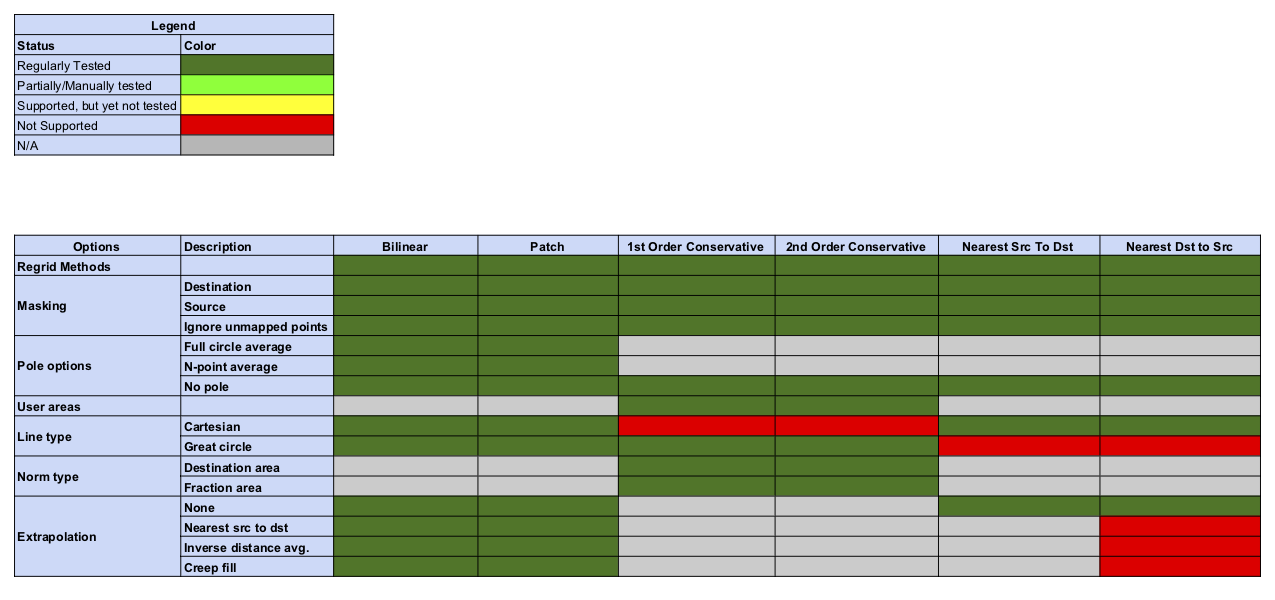
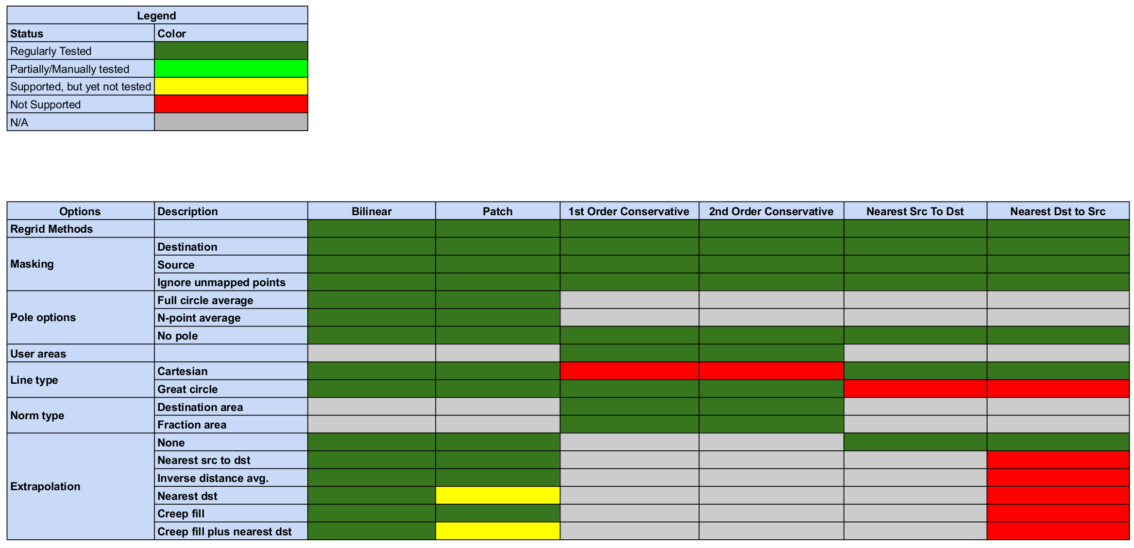
Status of Regridding Methods (covers releases 8.6.1/8.7.0/8.8.0/8.8.1/8.9.0/8.9.1)
There was no change in this release compared to 8.6.0.
Online (integrated) Regridding

Offline Regridding

Regridding Options Status

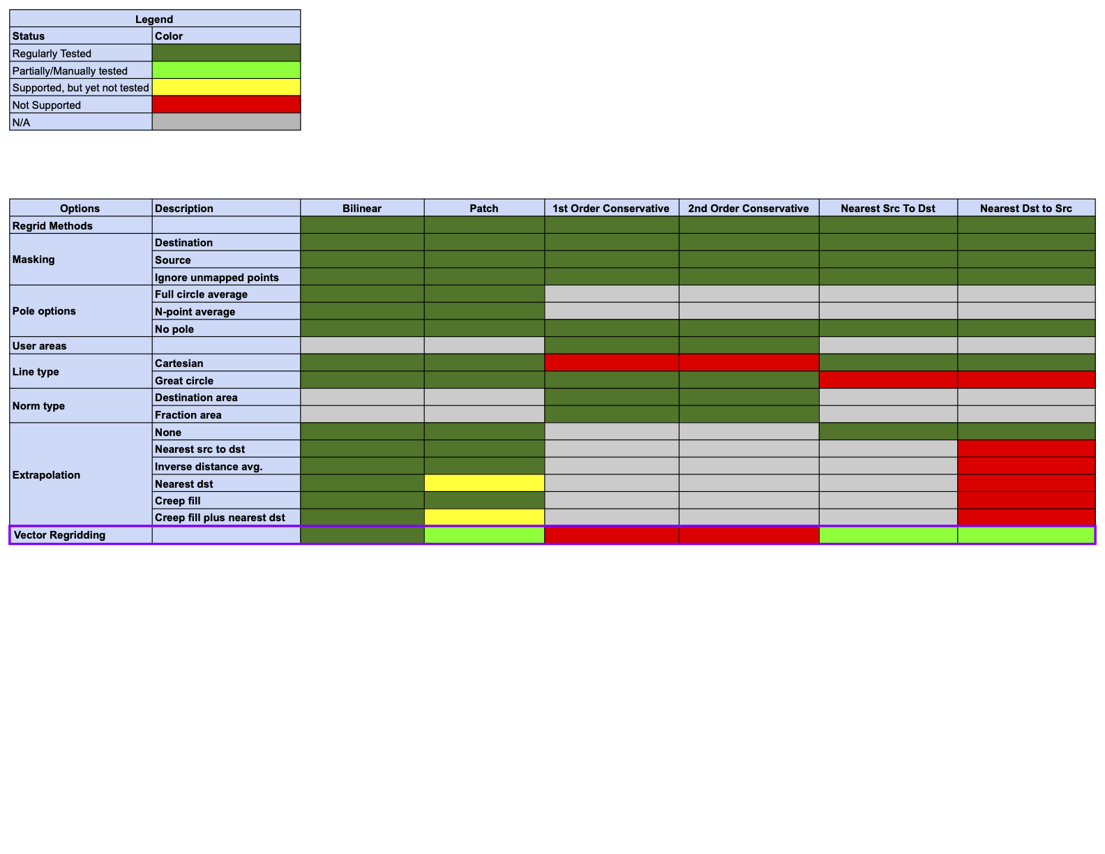
Status of Regridding Methods (covers release 8.6.0)
Changes compared to previous releases are indicated by a purple border in the status tables below. The only change with this release is the addition of the “Vector Regridding” option.
Online (integrated) Regridding

Offline Regridding

Regridding Options Status
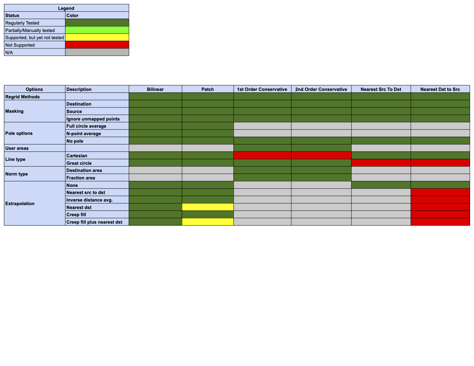
Status of Regridding Methods (covers releases 8.3.0/8.3.1/8.4.0/8.4.1/8.4.2/8.5.0)
Online (integrated) Regridding

Offline Regridding

Regridding Options Status
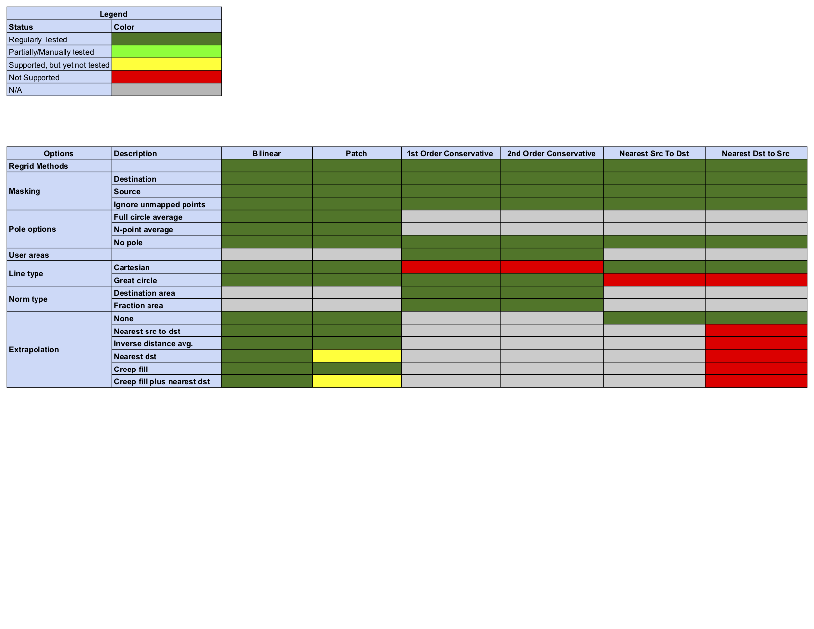
Status of Regridding Methods (covers release 8.2.0)
Online (integrated) Regridding

Offline Regridding

Regridding Options Status
Status of Regridding Methods (covers releases 8.1.0/8.1.1)
Online (integrated) Regridding

Offline Regridding

Regridding Options Status
Status of Regridding Methods (covers releases 8.0.0/8.0.1)
Online (integrated) Regridding

Offline Regridding

Regridding Options Status